Improvement of drought forecasting by means of various machine learning algorithms and wavelet transformation | Acta … – Springer

Droughts, which are generally divided into four categories, meteorological, agricultural, hydrological, and socioeconomic droughts, can cause different consequences depending on their type (Mishra et al. 2010; Wilhite and Glantz 1985). Meteorological drought which often affects water resources and available water availability is one of the most difficult to predict and detect. The frequency and percentage of meteorological droughts may vary from region to region depending on climate characteristics (Yaseen et al. 2021). Droughts present a complex challenge in climate science due to their multifaceted nature. Moreover, because droughts are directly linked to water availability, alterations in their characteristics resulting from climate change, and increasing temperatures of the water surface, will significantly affect water resources, food security, and dam management (Adnan et al. 2018). Although it is not easy to predict all challenging natural events, droughts are routinely observed and predicted using variety of drought indicators (DI) on a monthly or seasonal timescale (Hao et al. 2018).

Up to now, many methods have been developed by scientists interested in climate change to understand and monitor drought. One of the most popular of these indicators is the Palmer Drought Severity Index (PDSI) (Palmer 1965), which remained popular until the 1990s. It was subsequently replaced by the Standardized Precipitation Index (SPI), with its easier computability and applicability at different timescales. Despite some of its drawbacks which require at least 30 years of rainfall (Guttman 1994), SPI developed by McKee (1993) has become the most widely used drought indicator in the literature. Aside from SPI and PDSI, various drought indices, including the Standardized Runoff Index (SRI), the Standardized Precipitation Evapotranspiration Index (SPEI), the Standardized Hydrological Drought Index (SHDI), the Soil Moisture Drought Index (SMDI), and the Surface Water Supply Index (SWSI), are applicable for tracking both hydrological and meteorological drought conditions (Mishra and Singh 2011). These indicators have gained extensive use due to their simplicity and versatility in detecting, quantifying, and monitoring drought across various time frames (Jain et al. 2015; Jehanzaib et al. 2021; Kim and Jehanzaib 2020). It has been conducted by scientists to identify many droughts in terms of various regions. For example, Hinis and Geyikli (2023) discussed the accuracy of SPI predictions using several candidate distributions in Yeşilırmak, Kızılırmak, and Konya Closed Basins. They revealed that L-moments for the 3-month series and maximum likelihood approaches for the 12-month series were the strongest. Soydan Oksal (2023) in the Marmara region of Türkiye conducted a drought assessment related to the influence of temperature and precipitation using SPI and SPEI. According to the result, it required that temperature should be considered in future studies. Zeybekoglu (2022) conducted a drought assessment using SPEI on Hirfanli Dam Basin with metrological data including the precipitation and temperature data obtained from Gemerek, Kayseri, Kirsehir, Nevsehir, Sivas, and Zara meteorology observation stations located in Hirfanli Dam Basin between years 1968 and 2017. It was reported by Zeybekoglu that the most severe drought occurred in 2001 in Hirfanli Dam Basin. Berhail and Katipoğlu (2023) compared the agreement level between the Standardized Precipitation Index (SPI) and the Standardized Precipitation Evapotranspiration Index (SPEI) by means of the data compiled from the Mekerra Basin for 42 years from 1970 to 2011. They used Cohen’s kappa statistics and the Bland–Altman method to indicate the test of agreement between SPI and SPEI. In addition, the innovative trend analysis (ITA) method was employed.

It is paramount of important that droughts are detected, monitoring droughts even predicting for water resources management. Moreover, predicting drought several months or seasons ahead is crucial for lessening the adverse impacts of droughts (Dastorani and Afkhami 2011). Planning the future of water resources, managers can take precautions for this natural disaster. Many methods are used in the literature to forecast droughts in advance such as machine learning (ML) and stochastic processes. One of these methods the newest and the most innovative is ML. Rather than traditional methods, alternative machine learning is easily applicable, speedy, and flexible (Yaseen et al. 2021). In recent times, the scientific community has shown a growing interest in ML for research in various fields such as engineering, agriculture, medicine, marketing, as well as earth and environmental sciences. In particular, ML has influenced numerous areas of research due to high computational power and speed, readily available sensor data, and developments in big data analysis (Çoban et al. 2023). Due to the availability of big data in drought forecasts, many researchers have benefited from ML. Because of these, ML is thought to help a sustainable ecosystem (Deparday et al. 2019; Pérez-Alarcón et al. 2022; Pham et al. 2019).

Recently, many ML algorithms including artificial neural network (ANN), random forest (RF), and support vector machines (SVM) have been used in drought prediction modeling. Moreover, wavelet transform (WT) has been used to improve the performance of these models. For instance, with preprocessed WT Belayneh et al. (2014) compared SVM to ANN and found that the ANN models with WT (WA-ANN) performed better than WA-SVM in forecasting some SPI values in the Awash River Basin in Ethiopia. Deo and Şahin (2015) predicted drought with ANN considering SPEI in eastern Australia using predictive variable data from 1915 to 2012. According to the results, the multi-layer perceptron ANN model outperformed. Besides ANN, they used particle swarm optimization (PSO) and the response surface method (RSM) for SVM frequently used in the literature. Using many DI, such as SPI, Effective Drought Index (EDI) developed by Byun and Wilhite (1999), China-Z index (MCZI), Piri et al. (2023) assessed four machine learning algorithms, SVM-RSM, SVM-PSO, SVM, ANN, according to the results and described that SVR-PSO model was better than ANN, SVM in their results. Furthermore, they stated SVR-RSM produced superior abilities for both accuracy and tendency compared to other models. Mentioning crucial the prediction of hydrological droughts for available waters, Katipoğlu (2023b) used streamflow drought index (SDI) developed by Nalbantis (2008) for drought prediction modeling in the semi-arid Yesilirmak Basin. He benefited from a series of MI algorithms involving SVM, Gaussian process regression (GPR), regression tree (RT), ensembles of trees (ET), extreme gradient boosting (XGBOOST) and WT in his study. Performing coupled WT and artificial neural networks (WANN) models, Salim et al. (2023) used 39 discrete mother wavelets derived from five families including Haar, Daubechies, Symlets, Coiflets, and the discrete approximation of Meyer. They compared all discrete mother wavelets to each other and addressed that Meyer has the best forecast performance. Elbeltagi et al. (2023) anticipated SPI values in Jaisalmer, India, by merging the random subspace (RSS), M5 pruning tree (M5P), RF, and random tree (RAT) models. It has been discovered to boost M5P algorithms and the success of RSS. Recently, in addition to traditional methods, new methods have taken their place in the literature. Some of the most notable of these are: Pande et al. (2023) using the improved support vector machine model sequential minimal optimization (SVM-SMO) compared various kernel functions including SMO-SVM poly-kernel, SMO-SVM normalized poly-kernel, SMO-SVM PUK (Pearson Universal Kernel), and SMO-SVM RBF (radial basis function) kernel. They studied SPI at different time steps in the upper Godavari River Basin and stated that different kernel functions were successful according to the time steps. Estimating the groundwater level in Alabama, Robinson et al. (2024) used the long short-term memory (LTSM), one of the new machine learning methods, and WT benefiting from data, groundwater level, of 4 climate stations during 2011 and 2020 in their study. They stated that effective results were obtained in determining the groundwater level in the results and that the method used was quite sufficient for the estimations in the time series. They determined especially in the Cohen’s kappa statistic that there was a significant correlation between the results. Stating that drought is one of the most dangerous climate disasters, Achite et al. (2023b) used ELM and ELM with WT (W-ELM) to forecast the hydrological drought using data obtained from five stations and the standardized runoff index (SRI) at different time steps (1, 3, 6, 9, and 12 months) in Wadi Mina Basin (Algeria). The findings showed that the W-ELM model can be used for trustworthy drought forecasting in Algeria. Achite et al. (2023a) reported that the droughts, meteorological, hydrological, and agricultural, in the Mediterranean regions have raised concerns about the impact of climate change. Therefore, they emphasized that drought prediction modeling studies should be carried out and investigated droughts using a set of ML, the linear support vector machine (SVM), quadratic SVM, cubic SVM, fine Gaussian SVM, medium Gaussian SVM, coarse Gaussian SVM, rational quadratic Gaussian process regression (GPR), squared exponential GPR, Matern 5/2 GPR, exponential GPR, bagged tree, and boosted tree, in the Wadi Ouahrane Basin located in the regions. They also used 3 different DI, SPI, and SPEI and utilized WT. In the results, wavelet-GPR models showed the most promising results in estimating SPI, SPEI, and SRI values.

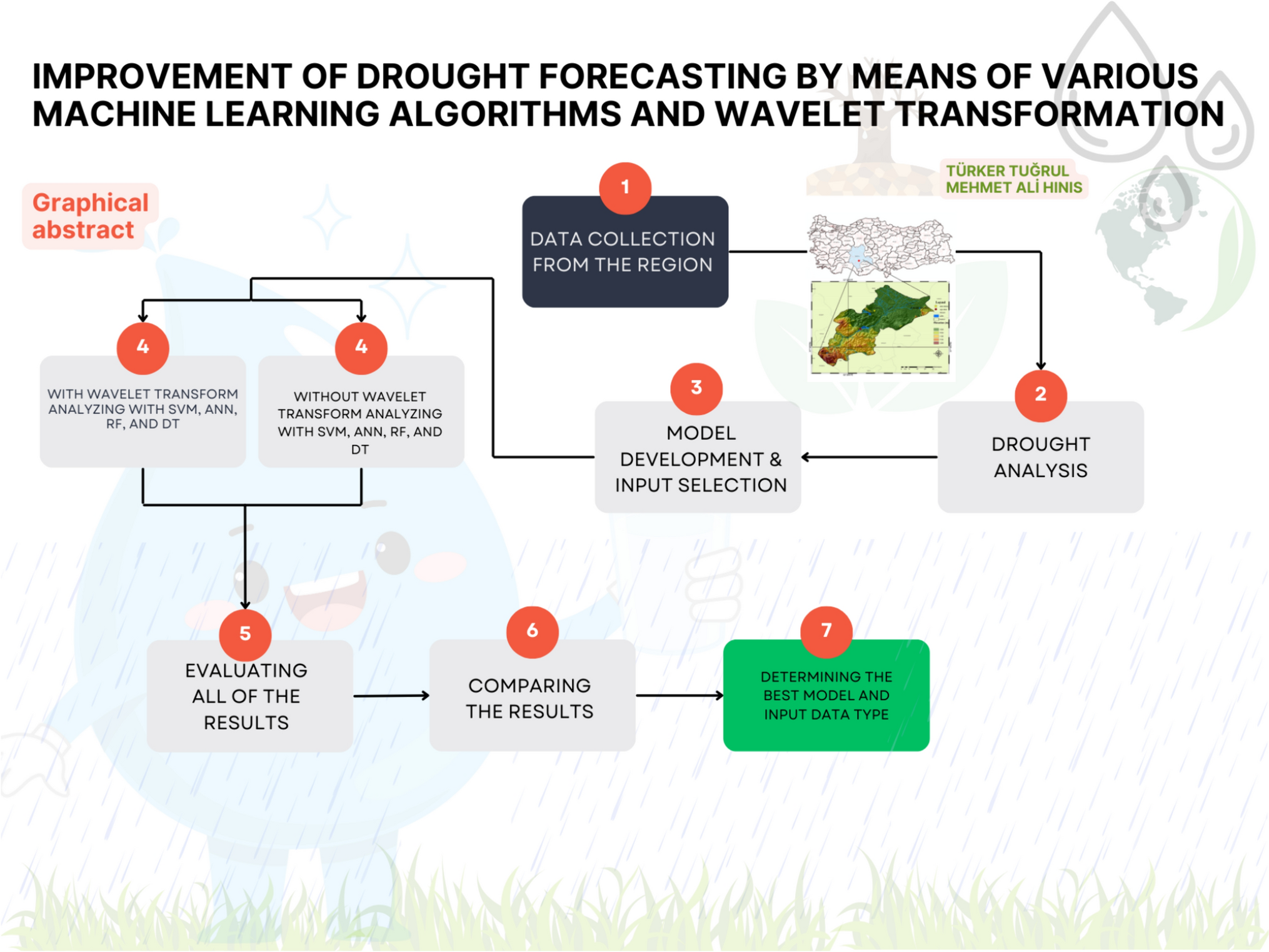
In many studies in the literature, two or three machine learning algorithms were generally used and the best model result was found according to the performance evaluation criteria. Most of the time, no work has been done to improve the results found with the traditional methods used. In this study, the Apa Dam Region located in the Konya Closed Basin of Turkey was examined and, unlike many previous studies, 4 different methods, SVM, ANN, RF, and DT, that are widely preferred in drought modeling in machine learning and are also preferred by many researchers in streamflow modeling were used for the study area in this study and WT was applied to improve the analysis result. In drought modeling studies, good models are generally established to represent the study area. However, no technique is applied by scientists to improve the performance of these established models. This is one of the main problems in drought modeling studies. In this study, we both researched the best model that could represent the region and improved the performance values of the model we built. Another problem encountered in drought modeling studies is the selection of data in the model input structure. Additionally, how many months the data used in the model inputs should be delayed and whether meteorological data will affect the model performance is one of the controversial issues in the literature. This is one of the problems we are trying to overcome. With this study, we aim to contribute to finding solutions to these issues. Additionally, this study aims to investigate the capabilities of different machine learning models by using meteorological data between 1955 and 2020 for the Apa Dam Region and find the best ML algorithm, SVM, ANN, RF, and decision tree (DT) using SPI. SPI is preferred in order to detect the drought, because SPI has advantages such as being easy to calculate, being able to produce results at different time steps, and only needing precipitation data in its calculation. Then, it is to find the best fitting model by applying WT to all models to improve the model results. Another aim of this study is to predict drought models in the future projection, to provide information to decision-makers about drought, which is one of the most dangerous among natural disasters, and to help them in developing strategies. The graphical abstract of this study is presented in Fig. 1.

Study area and data

Apa Dam whose construction and operation date back to the 1950s and 1965s is one of the important and large water resources of the Konya Closed Basin and is located in Çumra, Konya, Türkiye. Apa Dam, whose elevation is about 1000 m, built on Çarşamba water for irrigation and flood protection purposes has a maximum capacity of about 171,590 h m³ and is an earth fill type dam (Fig. 2). The dam is mainly fed by Bozkır-Çarşamba channel and Bağbaşı dam. The dam has an average surface area of 90,000 km². For this reason, the data for the dam were obtained from 3 different stations closest to the dam (Çumra, Bozkır, and Akören stations respectively). The available data from these stations are shown in Fig. 3. The monthly precipitation provided covers the period 1955–2022, and DI was calculated based on these data.

Standardized Precipitation Index (SPI)

SPI established by McKee et al. (1993) is widely used all over the world to identify droughts and rainfall deficiencies. This DI is designed to be used on different timescales (Kao and Govindaraju 2010). These timescales can also be used to describe short-term (for SPI3), mid-term (for SPI6), and long-term (for SPI12, 24-, 48) droughts (McKee et al. 1993). This calculation method works on the principle of equating long-term meteorological data with the gamma probability distribution and then converting it into a normal distribution (Edwards and McKee 1997). The following steps are followed in the calculation 1. The gamma probability function of long-term precipitation is calculated as in Eq. (1):

where (beta), (alpha), x, and (tau (alpha )) represent the scale, shape variables, rainfall amount, and gamma function, respectively. Equalities 2 and 3 determine the boundaries of (alpha) and (beta) (Guttman 1999):

where (overline{x}) and n denote the precipitation average and number of observations.

Equations (4) and (5) show the parameters used to derive the cumulative probability for nonzero rainfalls:

where:

Besides, the gamma function is undecided for x = 0. If this happens, the accumulative probability of zero and nonzero rainfall is calculated with Eq. (6) H(x):

For more detailed calculations, see McKee (1993), Edwards and McKee (1997), Mishra and Singh (2009).

Classification of the index values is given in Table 1 (McKee et al. 1993).

Artificial neural network (ANN)

Haykin (1998) mentioned an ANN as simple processors which are neurons that communicate with each other. Neurons store experimental information to obtain a logical conclusion. Similar to biological neural networks, this information is shared between neurons according to their weight and then a conclusion is reached. Finally, this process called learning in ANN is completed (Demuth and Beale 1998). The input layer allows the raw data to form a network and transfers the information obtained from this network to the result layer. There are many versions of ANN depending on these learning differences such as multi-layer perceptron (MLP) and feed-forward propagation (FFP). Due to its effective performance in hydrological forecasting (Piri et al. 2009), the ANN model applied in this study has a feed-forward MLP architecture trained using the Levenberg–Marquardt (LM) backpropagation algorithm.

Including a set of layers, as shown in Fig. 4, MLPs account for one input layer, one or more hidden layers and an output layer (Kim and Valdés 2003). It is briefly defined in Eq. (7). An ANN model’s structure with the signals transmitting layer by layer in a forward direction through the network is shown in Fig. 4 (Dikshit et al. 2020).

where m = number of hidden neurons, N = number of samples, x_i = ith input of variables at time step t; w_ji = weight which connects the ith and jth neurons in the input layer and in the hidden layer, respectively; b_j = bias for the jth hidden neuron; φ_j = activation function of the hidden neuron; w_j = weight that connects the jth and kth neurons in the hidden layer and in the output layer, respectively; b = bias for the kth output neuron; φ = activation function of the output neuron; and y is the predicted the kth output at time step t (Kim and Valdés 2003).

ANN calculations in this study were made with the help of the MATLAB program. Because it gave good results, among different activation functions such as linear, logistic, and sigmoid, the linear function was used for ANN in hydrology forecasting.

Support vector machines (SVM)

Used in classification and regression analysis, SVM introduced by Vapnik (1999) is widely used in forward-looking forecasts in hydrology as well as in many other fields. SVM works with the principle of statistical learning, and SVM provides an extraordinary solution for a given dataset, compared to other algorithms which may have different solutions. They provide effective results, especially in overfitting, by utilizing the kernel function used to estimate decision-making boundaries in nonlinear problems. If SVM is to be used in a regression, it can be referred to as SVR (Muller et al. 2001). While the main purpose of ANN is to minimize empirical risks, the main purpose of SVR is to ensure statistical learning minimization (Belayneh et al. 2014). SVM algorithm has demonstrated effectiveness in various applications within hydraulic engineering. These include estimating indicators for wastewater quality, predicting streamflow, modeling rainfall–runoff processes, assessing floods and droughts, as well as estimating sediment levels (Wang et al. 2018). SVM, which is generally used for regression purposes, is also frequently preferred for classification. It is one of the most successful algorithms in ML today, especially with its modifications. Many researchers use SVM and its modifications in their studies and stated that SVM and its modifications give effective results (Achite et al. 2023a; Katipoğlu et al. 2023). The SVR is counted by Eq. (8) by coupling between input and output:

where f(x) is a high dimensional feature space, w is a weight of the output variable, and b is the bias term.

Depending on the result performances, model results may differ by using kernel functions such as linear, poly, radial basis functions (RBF), sigmoid, and Gaussian. The Gaussian, which has the most impact on the model results, was used as the kernel function in this study. On the other hand, when the Gaussian is used, there are 3 different parameters that affect model performance results (ɣ) as the active function scale parameter, positive constant (C), and epsilon (ε) (Belayneh et al. 2016a). These parameters were automatically optimized in the MATLAB program to have the best effect on the model result while making calculations in this study. A detailed description of the theory and formulation of SVR can be found in Panahi et al. (2020), Vapnik (1999), Gunn (1998).

Random forest (RF)

Being a learning method an ensemble operated by constructing multiple decision trees, RF is frequently used in classification and regression processes. This method is created by combining many decision trees, and each tree works together in an ensemble rather than making a decision alone. RF is an ensemble learning technique designed to solve some of the basic problems of decision trees. Decision trees are widely used due to their many advantages: (1) High Performance: combining multiple decision trees generally provides higher performance than a single tree. (2) Less Preprocessing Requirements: generally, random forests can better deal with problems such as missing data and outliers. (3) Classification is one of the most effective ML methods. Each tree of RF is created from randomly selected samples. In addition to this randomness, ensemble learning is a major characteristic of RF (Biau and Scornet 2016; Breiman 2001). Taking into consideration a training dataset of N samples with M features, to create each tree, the randomness in RF can be expressed as randomly selecting each of the features. The bootstrap resampling method could be used to randomly form a sample set of size N. This process uses one-third of the data and is called out-of-bag data and the rest is called big data. By satisfying the m < M condition, random feature selection from the entire dataset is also applied as a subset. That is, a random selection subset (m) is created from the features of M. In general, the m parameter can be optimized according to the desired performance. This parameter may not be good in every study and one is often preferred in the literature (Yu et al. 2017). A detailed description of the theory and formulation of RF can be found in Breiman (2001), Oshiro et al. (2012), Yu et al. (2017).

Decision tree (DT)

DT, a nonparametric supervised learning method, is used in model development classification and regression. DT creates a model to predict the target variable by learning a set of it–then–else in a tree structure in a similar way. When using DT, the model is divided into various branches according to the targets to be detected, the process of breaking down the dataset into increasingly smaller subsets of similar or related types persists, akin to a divide-and-conquer algorithm, until a subset becomes homogeneous, indicating that the branch is sufficiently straightforward to make a direct decision. The procedure is repeated recursively until final nodes, which denote the result of following a combination of decisions, are reached. The outcome is a complex, branching structure akin to a tree, utilized for forecasting upcoming experiments. Decision trees are widely used due to their many advantages: (1) Simplicity: decision trees are generally easy to understand and easy to interpret. It is easy to visualize the structure of the tree and understand how it makes decisions. (2) Versatility: they can be used for both classification and regression problems. This means they can handle both categorical and continuous data types. (3) Importance of Features: decision trees can evaluate the importance of different features in the dataset and direct your model to focus on specific features. Its biggest disadvantage is that it falls into excessive memorization. In DT, some algorithms such as classification and regression trees (CART), C5.0, quick unbiased efficient statistical tree (Quest), and Chi-squared automatic interactive detector (CHAID) are used according to these tree branches or nodes. In this study, the CART algorithm, developed by Breiman (1984), was used because it had a positive effect on the model result.

Discrete wavelet transformation

Wavelet transform is generally faced in two ways in the literature: continuous wavelet transformation (CWT) and discrete wavelet transformation (DWT). Due to the computational difficulties in CW implementation, DWT is generally preferred over CWT (Kisi 2011).

DWT serves as an alternative to the Fourier transform, employing a signal processing technique that decomposes time series into distinct sub-signals across different frequencies, ultimately providing the desired characteristics (Maheswaran and Khosa 2012; Sang 2013). It is a practical mathematical function that gives a time–frequency description of a signal analyzed in the time domain. A wavelet function (psi_{y} (t)), the mother wavelet, is a small wave that distinguishes distinct frequencies. It is performed at various scales ((s_{0})) and localized around time ((tau_{0})). The mother wavelet is calculated in Eq. (9):

where m and n are integers that control the scale and time; ψ(t) is. Then, the most frequent choices for the parameters S₀ and (tau_{0}) are 2, 1 respectively. According to Mallat’s theory (1989), the irreplaceable discrete wavelet transform (DWT) can break down into inverse DWT a sequence of approximation and detail signals that are linearly independent. (s_{0}) represents the step of precision expansion, and (tau_{0}) represents the location parameter DWT for a discrete time series x_i, in which x_i happens at discrete time i. Equation (10) gives the inverse DWT as per Mallat (1989):

where (W_{m,n} 2^{{ – frac{m}{2}}} sumnolimits_{t = 0}^{N – 1} {psi left( {2^{ – m} t – n} right)x(t)}) is the wavelet coefficient for the discrete wavelet at scale (s = 2^{m}) and (tau = 2^{m}) n. In this study, we preferred five-level detailed studies in wavelet transform because it improved the model results. The calculation for the level is made as Eq. (11):

where L is the level of the decomposition and N is the number of runs.

Model performance criteria

There are various statistical performance measurements criteria in the literature. The created models were appraised to test the prediction accuracy of models with 3 different statistical methods: correlation coefficient (R) (Eq. 11), RMSE (root mean square error) (Eq. 12), and Nash–Sutcliffe efficiency (NSE) coefficient (Eq. 13). In Eqs. (11–13), ({text{SPI}}_{pi}) = the predicted value, ({text{SPI}}_{oi}) = the observed value, N = the number of data, (overline{{{text{SPI}}_{o} }}) = average observed value, and (overline{{{text{SPI}}_{p} }}) = average predicted value.

Correlation coefficient (R) is given in Eq. (12) (Khan et al. 2020):

RMSE is given in Eq. (13) (Zhang 2017):

NSE is sensitive to additive and proportional differences between forecasts and observations (Nash and Sutcliffe 1970).

NSE is calculated in Eq. (14):

Model structure

In the literature, it is found that the 3- and 12-month time periods of SPI better represent agricultural and hydrological drought, respectively (Mohammed et al. 2022). So, instead of performing a study on all time steps of the SPI, the 3- and 12-month timescales of the SPI were used in this study. In addition to these time steps, we also added 6- and 9-month time steps to this study to conduct a more comprehensive study. Information on all models used in this study is shown in Table 2. Additionally, we preferred the model input structure consisting of a single data type, only SPI, which is frequently used in the literature (Katipoğlu 2023a; Khan et al. 2020) and added the precipitation data to the input structure of M05 for differences.

Here P = monthly precipitation. While creating the models, the output structure was determined as SPI for time t. The input structures were created with SPI data delayed at different times, with delays of 4, 5, 6 months. It has been thought that the monthly precipitation data for time t − 1 may also affect the model output results. Subsequently, it was added to the input structures of models, M04, M08, M12, M16.

In this part of the study, all models were analyzed with different algorithms, ANN, SVM, RF, DT, and the results of all models obtained from these analyses were mentioned. Additionally, the results were improved with wavelet transform. When analyzing with algorithms, 70% of the data were determined as learning set while 30% of the data for test set. Moreover, all model results in two different situations, before and after wavelet transform, were compared with each other. The result is provided from the prediction of the test dataset.

Drought analysis

The time series of all calculated SPI values (SPI3, 6, 9, 12) are shown in Fig. 5. It has been determined that in short periods dry–wet period transitions are higher than in long periods. While it was observed in dry periods that the index value reached as low as 2.5 in SPI12, the lowest index value increased above − 3 in SPI9. During wet periods, the highest index value was again found in SPI9. Extremely dry periods for SPI12 were observed in December 1956, January 1957, and October 2016; for SPI9 November 1956 and December 1999; for SPI6 November 1956, September 1966, September 1984, November 1999, and September 2012; and for SPI3 August 1962, September 1964, 1966, 1972, and 1993, October 2004, and September 2010 and 2017.

Performance of the models before applying wavelet transform

Performance evaluation results of analyses carried out with different algorithms are given in Table 3. According to this table, analyses performed with SVM provided superior performance compared to other algorithms in almost all models.

As a result of the analysis carried out with SVM, the high NSE value and the lowest RMSE value were found in M04. The performance values of M04 are NSE = 0.8694, RMSE = 0.3610, R = 0.9329. The input structure of M04 was created from SPI12 data delayed up to 5 months and monthly precipitation data for time t − 1. Apart from M04, another high result in SPI12 was detected in M03. The input structure of M03 was created from SPI12 delayed for up to 6 months. The performance values of M04 and M03 are almost the same. Another striking finding in Table 3 is that as the number of steps of SPI increases, model performances also increase. Looking at the results of the models where SPI9 was used as input data, it was determined that the most successful result was obtained in M05 and M06. The input structure of M05 was created from SPI9 data delayed by up to 4 months and M06 for 5 months. The performance values of models are NSE = 0.8040, RMSE = 0.4355, R = 0.8967: NSE = 0.8043, RMSE = 0.4359, R = 0.8969, respectively. These values are very close to each other. Unlike SPI12, the best performance values in SPI9 were calculated in models whose input data were created only with the SPI index. Because when it comes to SPI6, as the number of steps decreases, the difference in performance values between models increases and the most successful model can be identified more clearly. The best performance values in this section were found to be M09 (NSE = 0.7620, RMSE = 0.4821, R = 0.8748) and M10 (NSE = 0.7646, RMSE = 0.4805, R = 0.8760). The input structure of these models was created from SPI6 data delayed up to 4 and 5 months, respectively. Here, it was determined that delaying the input data for time 6 months negatively affected the model performance. The most successful model in SPI3 was determined to be M16 (NSE = 0.6255, RMSE = 0.5831, R = 7951). The input structure of M16 was created from SPI12 data delayed up to 5 months and monthly precipitation data for time t − 1.

In the analysis carried out using ANN, the most successful result both in general and in SPI12 was found in M01 (NSE = 0.8515, RMSE = 0.3824, R = 9233) whose input structure of M01 is created from SPI12 data delayed by up to 4 months. In SPI9, the most successful result was determined in M05 that created input structure with SPI9 data delayed up to 4 months. In SPI6, another data used in ANN, the model with the best performance, compared to other model results, is M09 (NSE = 0.7438, RMSE = 0.5002, R = 8650), and input structure of this model consists of SPI6 data delayed up to 4 months. Finally, the most effective model in SPI3 was determined to be M13 which be input data the same as M09. The most striking finding is that, in general, only SPI data are used in the input structure of models that are successful in ANN.

When the analyses used by RF were examined, in SPI12, it was determined that the most successful result was obtained in M01 (NSE = 0.8406, RMSE = 0.3962, R = 9183), as in SVM and ANN. In SPI9, although the results of M05, M06 and M08 were close to each other, it was calculated that M05’s performance values were slightly better than the others. Besides, the input structure of this model consists of SPI9 data delayed up to 4 months. Although all results in SPI6 obtained with 6-month precipitation totals are very close to each other, one of them (NSE = 0.7549, RMSE = 0.4892, R = 0.8691), M09, including in input structure from SPI6 data delayed up to 4 and 5 months, is the best performer. The model that performs best in SPI3 is M16. While adding monthly precipitation data as input to the model structure in RF had little effect on SPI6, it had a positive substantial impact on the model result in SPI3.

When we look at the group in DT, M04 consisting of input structure delayed SPI12 up to 5 months and monthly precipitation data for time t − 1 exhibited better performance than others (NSE = 0.8342, RMSE = 0.4067, R = 0.9147). As in other algorithms, model performance values in this class are very close to each other. But, compared to other algorithms, the lowest performance values in the SPI12 class were detected in DT. Analyses carried out using SPI9 data show that M08 performs better than M07, M06 and M05. The input structure of M08 was created from SPI9 data delayed up to 5 months and monthly precipitation data for time t − 1. Here, monthly precipitation data had a positive impact on the model result. Finally, M13 (NSE = 0.4930, RMSE = 0.6852, R = 0.7073) and M09 (NSE = 0.7335, RMSE = 0.5101, R = 0.8577) performed better at SPI6 and SPI3, respectively, than other models.

In the comparison of all models made with different algorithms, the 2 most successful models in their group for each algorithm are shown in the violin diagram in Fig. 6. When Fig. 6 is examined, no pattern similar to the observation pattern could be detected. However, it is shown in the diagram that SVMM04 and SVMM03 are partially similar. Consequently, in this part of the study conducted without wavelet transform, 4 different machine learning algorithms, SVM, RF, ANN, and DT, were compared with each other, and although the results were close to each other, SVM gave the best result, where SVM = used ML, M04 = model name. Figure 6 shows that the results of other models do not match the observation values.

The harmony between the results of the most successful models and observation values in time series is shown in Fig. 7. When examined, it was determined that ANN M01 did not fully match the observation values and could not fully capture the peaks. In Fig. 7, however, it was clearly seen that in SVM M04, the results closest to the observation values were obtained and the peak points were detected. Therefore, the most successful results were found in M01 with the SVM algorithm.

Figure 8 shows the comparison of observation values and results of the most successful models in DT and RF. It was found that both models could not capture the peak values of the observation values. It was indicated that DT fell into memorization at some points.

Performance of the models after applying wavelet transform

Performance evaluation results of analyses carried out with different algorithms are given in Table 4. According to this table, analyses performed with SVM had superior performance to the other algorithms in almost all models compared to others. The first impressions in wavelet transform are that there are improvements in model results in ANN and SVM. But, this improvement is not at a very good level in RF and DT. It even brought about a negative impact on some model results.

According to the analysis results using SPI12 as input data in SVM, better NSE, RMSE, and R values were obtained in M04 whose input structure of not only SPI12 data but also meteorological data were used in the input structure of M04 (NSE = 0.9942, RMSE = 0.0764, R = 0.9971) compared to the others, M01, M02, M03. Adding meteorological data, monthly precipitation data, to the input data positively affected the model result. When looking at the performance values of models using SPI9 as input data in SVM, here the most effective result was obtained in M06 (NSE = 0.9915, RMSE = 0.0908, R = 0.9958). SPI9 data delayed up to 5 months were used in the input data of M06. So, it can be concluded from this that delaying for the optimum time is crucial. Whereas in SPI6 all results are very close to each other in SVM, in SPI3 the results are slightly apart and M16 (NSE = 0.9772, RMSE = 0.1438, R = 0.9887) exhibited the best result in SPI3. Just as in SPI12, when it was used meteorological data, a slightly better result was obtained than the results of other models changed with input structure using only SPI3.

When we looked at the results obtained with ANN, in models that use SPI12 as input data, the best results were obtained in M04 (NSE = 0.9698, RMSE = 0.1735, R = 0.9849) created both SPI12 and meteorological data of monthly precipitation. The M05 (NSE = 0.9749, RMSE = 0.1557, R = 0.9879) model appears to be the model that gives the best results among the models in which SPI9 is used as input data in Table 4. The input structure of this model was created with SPI9 data delayed up to 4 months. The low number of delays had a positive effect on performance criteria parameters. Another successful model is M09 with NSE = 0.9626, RMSE = 0.1911, and R = 0.9832 in his own group, in SPI6. It was understood from M09 that keeping the number of delayed months, SPI6, in the input data at an optimum level affected the model server positively. In SPI3, the most successful result was obtained in M16. Meteorological data were used in the input structure of this model, monthly precipitation.

As a result of the analysis carried out with the RF and DT algorithms, it was determined that the wavelet transform reduced the model performances. SPI3 data were used in the input data of M13, M14, M15, and M16. For this reason, the performance values of these models are lower than the others. While the model performances in SVM and ANN decrease as the time steps of SPI decrease, the opposite happens in RF and DT. While WT had a positive effect on the models created with SPI3 in RF and DT, it had a negative effect on other steps of SPI. In both algorithms, the best result was obtained in M16 which used SPI3 and monthly precipitation data in the input structure.

Comparisons between the models were made in the previous section. Here comparison of ML algorithms with each other was mentioned. Therefore, when comparing models with each other, the model results in SPI12, which is generally the most successful, were taken into account. Figure 9 demonstrating all model performances with wavelet in violin diagram shows the similarity of all machine learning with observation values. By using this picture, machine learning algorithms could be compared with each other. It appears that the model that gives the closest result to the observation values is SVMWM04, where SVM = used ML, W = being wavelet transform, M04 = model name. Figure 9 shows that the results of other models fully do not match the observation values.

As a result of the analysis carried out with wavelet transform, according to time series and observation values, the most successful model results are shown in Fig. 10. This figure shows that both models are in perfect agreement with the observation values. However, it was determined that very good predictions were not made at the beginning of the observation values of ANN. Therefore, SVM M04 was determined as the most successful model.

Figure 11 shows the time series of the most successful models in DT and RF. Figure 11 shows the time series variation of the results obtained from the most successful models in DT and RF. It was determined that the results of both models did not match the observation values. It was indicated that the model performances were low and poor.

ANN and SVM have started to be used for a while. Both of these methods are very popular in drought modeling studies and provide better results than the other methods such as Naive Bayes. Recently, RF and DT methods have been added to these methods. Whereas ANN and SVM are generally preferred for regression models, RF and DT are preferred for classification problems. It is emphasized in the literature that RF gives better results than SVM. Based on all these inferences, these methods were chosen in this study to obtain the best results.

When similar results were obtained in some studies in previous drought forecasting studies using ML, Achite (2023a) mentioned in their results that ML models with WT superior over other ML models without WT and the results could guide decision-makers, government, and planners in developing natural risk management. Preferring to work with SVM and ANN, WT and the bootstrap, Belayneh et al. (2016b) tried to predict drought using precipitation in the Awash River Basin, located in Ethiopia. They stated that WT was more effective than the other methods. Katipoğlu et al. (2023) expressed the importance of modeling studies in planning water resources and combating drought in their study. They used new hybrid approaches, combining least square support vector machines (LSSVM), empirical model decomposition (EMD), and PSO, for modeling in the study. They stated that SVM modification models, PSO-LSSVM and EMD-LSSVM, were successful as a result of the study carrying out using the streamflow data between 1964 and 2005 in the Konya Closed Basin. Piri et al. (2023) studied various ML models, modifications of SVM and ANN, generally hybrid methods, to predict the droughts in Iran. They mentioned the effective and widespread use of hybrid methods recently, and SVM-SPO and SVM-RSM are more effective than ANNs.

In this study, droughts were analyzed with monthly precipitation data in the Apa Dam region and drought prediction models to predict future potential droughts were created for this region with machine learning algorithms, SVM, ANN, RF, and DT. In addition, wavelet transform was applied to improve the model results. For the region, the most effective model structure was researched and the most useful machine learning algorithm was determined. The most striking results of the research are as follows:

• SVM exhibited the most effective performance both in wavelet transform and without wavelet transform. In all analyses, both without wavelet and with wavelet, performed with SVM, adding monthly precipitation data to the model input structure in SPI12, SPI3 affected positively the model result, rather than just only using SPI data. It was determined that models with only drought indices in SPI6 and SPI9 showed effective performance. It was also determined that the number of delayed months would be kept at the optimum level which is 4 rather than 5, 6 in SPI6 and SPI9. After wavelet transform, the most effective result in SVM was obtained in M04 as before transformation. Successful models remain unchanged after the transformation, and M06 in SPI9, all of them in SPI6, and M16 in SPI3 showed effective results.

• ANN is the most effective machine learning algorithm after SVM. In ANN, using meteorological data as input data generally had a negative impact on model results. Furthermore, because effective results were obtained in models created only with SPI value, it was concluded that the delayed SPI data in the model input structure in SPI12, SPI9, SPI6 should be kept at the optimum level, that is, up to 4 months. After wavelet transform, whereas the most effective result in SPI12 was obtained in M04 created input data delayed up to 5 months and monthly precipitation data for time t − 1, SPI9 for M05 created only delayed up to 4 months. In SPI6, the most successful result was obtained in M09 whose input data were delayed up to 4 months.

• In RF, effective performances were obtained in models where model input was created only SPI value all SPI time steps except for SPI3. Moreover, successful the results were obtained in the model created with a monthly precipitation data in SPI3. Model performances after wavelet transform in RF and RF are generally poor.

• DT exhibited the worst results among all algorithms both without wavelet transform and with wavelet transform.

• Although DT and RF are good at regression and especially classification without wavelet transform, wavelet transform generally had a negative effect. But in models created with SPI3, M13, M14, M15, and M16, this effect is positive.

• Using RF and DT with wavelet transform, which are good in classification algorithms, may cause negative effects in regression analysis.

The findings of the study offer improved estimates for the drought and valuable insights for water-related institutions and organizations responsible for managing water resources and addressing meteorological-based natural disasters like floods and droughts. Due to its geographical location, Konya Closed Basin suffers greatly from precipitation deficiencies and consequent droughts. The scarcity of forests in the regions also triggers droughts. Considering that most of Türkiye’s grain needs are met from this region, the results of this study are thought to be helpful to decision-makers.

Recommendations for future studies can be listed as follows: (1) In terms of the methods used, although SPI is used, which seems to be a method that will never lose its popularity, different the drought index calculation methods can be used. (2) By adding the data such as evaporation and temperature to the model data, it is considered appropriate to conduct a drought modeling study using a few more stations close to the region. (3) If possible, more meteorological stations can be established in the region and a more detailed drought modeling study can be carried out.

With this study, we investigated a model and methods that we think may be useful in predicting possible droughts for decision-maker authorities for people who live in the region and engage in agriculture and who may also suffer from the drought. We think that if the results we obtain here are adopted or accepted by the relevant institutions, precautions can be taken against possible the droughts.

The main limitation of the study is that it combines a series of machine learning (SVM, ANN, RF, and DT) with the wavelet transform method and the data type is small. Perhaps more realistic results can be obtained with a wider variety of data and different learning algorithms by applying preprocessing methods to the data.